Time Synchronization
Papers referenced:
"Timing-sync Protocol for Sensor Networks" by Ganeriwal, Kumar, and Srivastava
"Fine-Grained Network Time Synchronization using Reference Broadcasts" by Elson, Girod, and Estrin
Overview
Generally, timing is a challenging an important issue in building
distributed systems. Consider a couple of examples:
- A distributed, real time auction where the system must know which of two bidders submitted their bid first.
- A TDMA protocol that requires coordination among sensor nodes.
- A MAC protocol that requires coordination among sensor nodes.
- An application that determines the angle of arrival of an
acoustic signal by analyzing the times at which the signal reaches an
array of sensors.
In some cases, it may be sufficient to know the order in which events
occur. This is referred to as logical time. In other cases,
it is necessary that two computing devices be synchronized with respect
to physical time.
Clock Synchronization
Every computer has a physical clock that counts oscillations of a crystal.
This hardware clock is used by the computer's software clock to track the
current time. However, the hardware clock is subject to drift
-- the
clock's frequency varies and the time becomes inaccurate. As a result,
any
two clocks are likely to be slightly different at any given time.
Ganeriwal reports that motes can lose up to 40 microseconds every
second. The
difference between two clocks is called their skew.
There are several methods for synchronizing physical clocks. External
synchronization means that all computers in the system are synchronized
with an external source of time (e.g., a UTC signal). Internal
synchronization means that all computers in the system are synchronized
with one another, but the time is not necessarily accurate with respect to
UTC.
In a system that provides guaranteed bounds on message transmission time, synchronization is straightforward since upper
and lower bounds on the transmission time for a message are known. One
process sends a message to another process indicating its current time,
t. The second process sets its clock to t + (max+min)/2
where max and min are the upper and lower bounds for the message transmission
time respectively. This guarantees that the skew is at most
(max-min)/2.
Cristian's method for synchronization in systems that do not provide such guarantees is similar,
but does not rely on a predetermined max and min transmission time. Instead,
a process p1 requests the current time from another
process p2 and measures the RTT
(Tround) of the request/reply. Whenp1
receives the time t from p2 it sets its time to
t + Tround/2.
The Berkeley algorithm, developed for collections of computers running
Berkeley UNIX, is an internal synchronization mechanism that works by
electing a master to coordinate the synchronization. The master polls the
other computers (called slaves) for their times, computes an average, and
tells each computer by how much it should adjust its clock.
The Network Time Protocol (NTP) is yet another method for
synchronizing
clocks that uses a hierarchical architecture where he top level of the
hierarchy (stratum 1) are servers connected to a UTC time source such
as a GPS unit. The TPSN protocol is very similar to NTP.
Synchronization in WSN
Some classifications of synchronization protocols:
- Physical time versus logical time
- External versus internal synchronization
- A priori versus posteriori synchronization - post-facto
synchronization in WSN has been proposed in several papers.
Post-facto synchronization happens on demand, after the event
occurs. In this way, synchronization -- which requires resources
such as energy -- only happens when necessary.
Performance metrics:
- Precision - synchronization error
- Energy cost
- Memory requirements
- Fault tolerance
- Scalability
Decomposition of packet delay:
- Send time - Time for the packet to pass from the application
layer to the MAC layer -- highly variable based on delays introduced by
OS.
- Access time - Time the MAC layer must wait for the channel to
become free -- highly variable based on make protocol and one of the
most critical factors contributing to delay.
- Transmission time - Time to transmit entire packet -- mainly
deterministic and can be estimated based on packet size and radio speed.
- Propagation time - Time to traverse the link -- typically negligible in WSN.
- Reception time - Time for the receiver radio to receive bits and pass to MAC layer -- mainly deterministic.
- Receive time - Time for MAC layer to construct packet and send to application layer -- changes based on delays of OS.
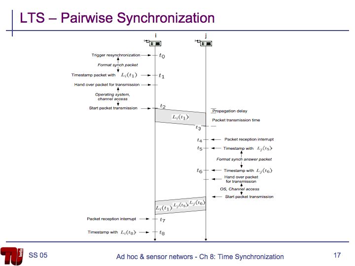
To reduce the delay at the sender (send time + access time +
transmission time) and receiver (reception time + receive time), most
time synchronization protocols propose the use of timestamps taken at
the MAC layer.
TPSN Overview
TPSN is a sender-receiver synchronization algorithm that works similarly to NTP.
- Level Discovery - Create
a hierarchical topology in the network, similar to NTP. The root
node at level 0 may be synchronized with UTC time, for example using a
GPS receiver.
- Synchronization Phase - nodes at level i synchronize to a node at level i-1.
Level Discovery
- Root broadcasts a level_discovery packet containing the level and identity of the sender.
- Receivers assign themselves a level one greater than the level of the sender.
- Receivers broadcast a new level_discovery packet containing their level.
- Once a node is assigned a level it ignores future level_discovery packets.
Synchronization Phase
- Use sender-receiver synchronization to synchronize nodes at level i with nodes at level i-1.
- At time T1 node A sends a synchronization_pulse to node B. The packet contains A's level and the value T1.
- Node B receives the packet at time T2 and sends an ACK at time T3. This packet contains the values T1, T2, and T3.
- Node A receives the ACK at time T4.
- Assuming that clock drift and propagation delay do not change between T1 and T4, the clock drift can be calculated as:
- The propagation delay can be calculated as:
- The root initiates synchronization by broadcasting a time_sync packet.
- Receivers at level 1 wait for a random amount of time (to avoid collision) and send the synchronization_pulse to the root.
- Nodes at level 2 will hear the synchronization_pulse of nodes at
level 1, backoff for a random time, and send a synchronization_pulse.
Special Provisions
- Nodes can proactively join the network by sending a level_request
message. Neighbors respond and the requesting node can assign
itself a level.
- If a node's parent dies, the node will eventually timeout and send a level_request to rejoin the network.
- If the root dies, the remaining nodes can execute a leader
election algorithm and the elected leader will take over the
responsibilities of the root.
Reference-Broadcast Synchronization (RBS)
RBS is a receiver-receiver synchronization algorithm that is an
alternative to TPSN. In RBS, nodes send reference beacons that
are heard by other nodes within broadcast range. These nodes then
use the time the broadcast is received to synchronize their clocks.
- A sender broadcasts a reference packet.
- Receivers i and j in the same broadcast domain receive the broadcast and record their local times.
- Receivers i and j exchange their observations to determine the offset of their clocks.
Logical Time
Physical time cannot be perfectly synchronized. Logical time provides a
mechanism to define the causal order in which events occur at
different processes. The ordering is based on the following:
- Two events occurring at the same process happen in the order in which
they are observed by the process.
- If a message is sent from one process to another, the sending of the
message happened before the receiving of the message.
- If e occurred before e' and e' occurred before e" then e occurred
before e".
"Lamport called the partial ordering obtained by generalizing these two
relationships the happened-before relation." ()
In the figure, and . Also, and , which means that . However, we cannot say that or vice versa; we say that they are concurrent
(a || e).
A Lamport logical clock is a monotonically increasing software counter,
whose value need bear no particular relationship to any physical clock.
Each process pi keeps its own logical clock,
Li, which it uses to apply so-called Lamport
timestamps to events.
Lamport clocks work as follows:
- LC1: Li is incremented before each event
is issued at pi.
- LC2:
-
- When a process pi sends a message m,
it piggybacks on m the value t =
Li.
- On receiving (m, t), a process pj
computes Lj := max(Lj, t) and then
applies LC1 before timestamping the event receive(m).
An example is shown below:
If then L(e) < L(e'), but the converse is not true. Vector clocks
address this problem. "A vector clock for a system of N processes is an array
of N integers." Vector clocks are updated as follows:
VC1: Initially, Vi[j] = 0 for i, j = 1, 2, ..., N
VC2: Just before pi timestamps an event, it sets
Vi[i]:=Vi[i]+1.
VC3: pi includes the value t = Vi in every message
it sends.
VC4: When pi receives a timestamp t in a message, it sets
Vi[j]:=max(Vi[j], t[j]), for 1, 2, ...N. Taking the
componentwise maximum of two vector timestamps in this way is known as a
merge operation.
An example is shown below:
Vector timestamps are compared as follows:
V=V' iff V[j] = V'[j] for j = 1, 2, ..., N
V <= V' iff V[j] <=V'[j] for j = 1, 2, ..., N
V < V' iff V <= V' and V !=V'
If then V(e) < V(e') and if V(e) < V(e') then .
Global States
It is often desirable to determine whether a particular property is true
of a distributed system as it executes. We'd like to use logical time to
construct a global view of the system state and determine whether a
particular property is true. A few examples are as follows:
- Distributed garbage collection: Are there references to an object
anywhere in the system? References may exist at the local process, at
another process, or in the communication channel.
- Distributed deadlock detection: Is there a cycle in the graph of the
"waits for" relationship between processes?
- Distributed termination detection: Has a distributed algorithm
terminated?
- Distributed debugging: Example: given two processes p1 and
p2 with variables x1 and x2
respectively, can we determine whether the condition
|x1-x2| > δ is ever true.
In general, this problem is referred to as Global Predicate
Evaluation. "A global state predicate is a function that maps from the
set of global state of processes in the system ρ to {True, False}."
- Safety - a predicate always evaluates to false. A given undesirable
property (e.g., deadlock) never occurs.
- Liveness - a predicate eventually evaluates to true. A given desirable
property (e.g., termination) eventually occurs.
Cuts
Because physical time cannot be perfectly synchronized in a distributed
system it is not possible to gather the global state of the system at a
particular time. Cuts provide the ability to "assemble a meaningful global
state from local states recorded at different times".
Definitions:
- ρ is a system of N processes pi (i = 1, 2, ..., N)
- history(pi) = hi = <, ,...>
- =<, ,..., > - a finite prefix of the process's history
- is the state of the process pi immediately before the
kth event occurs
- All processes record sending and receiving of messages. If a process
pi records the sending of message m to process pj
and pj has not recorded receipt of the message, then m is part
of the state of the channel between pi and pj.
- A global history of ρ is the union of the individual
process histories: H = h0 h1 ∪ h2
∪...∪hN-1
- A global state can be formed by taking the set of states of
the individual processes: S = (s1, s2, ...,
sN)
- A cut of the system's execution is a subset of its global
history that is a union of prefixes of process histories (see figure
below).
- The frontier of the cut is the last state in each process.
- A cut is consistent if, for all events e and
e':
- ( and )
- A consistent global state is one that corresponds to a
consistent cut.
Distributed Debugging
To further examine how you might produce consistent cuts, we'll use the
distributed debugging example. Recall that we have several processes, each
with a variable xi. "The safety condition required in this example
is |xi-xj| <= δ (i, j = 1, 2, ..., N)."
The algorithm we'll discuss is a centralized algorithm that determines
post hoc whether the safety condition was ever violated. The processes in the
system, p1, p2, ..., pN, send their states
to a passive monitoring process, p0. p0 is not part of
the system. Based on the states collected, p0 can evaluate the
safety condition.
Collecting the state: The processes send their initial state to a
monitoring process and send updates whenever relevant state changes, in this
case the variable xi. In addition, the processes need only send
the value of xi and a vector timestamp. The monitoring process
maintains a an ordered queue (by the vector timestamps) for each process
where it stores the state messages. It can then create consistent global
states which it uses to evaluate the safety condition.
Let S = (s1, s2, ..., SN) be a global
state drawn from the state messages that the monitor process has received.
Let V(si) be the vector timestamp of the state si
received from pi. Then it can be shown that S is a consistent
global state if and only if:
V(si)[i] >= V(sj)[i] for i, j = 1, 2, ..., N
Sami Rollins
Date: 2008-01-15