Create by hand a neural network that takes 3 binary inputs, and returns 1 if and only exactly 2 of the inputs are on and false otherwise. You will likely need a 2-layer model. You do not need to try to build this from data. You can turn in a pictorial drawing, or something text-based -- a text-based solution to the XOR problem defined in class would be:
2 Inputs, I1 and I1
2 Hidden nodes H1 and H2
1 Outut Node O1

H1 weights:  Bias -1, from I1 0.6, from I2 0.6
H2 Weights:  Bias -0.04, from I1 0.5, from I2 0.5

O1 Weights:  Bias -0.3, from H1 -0.4, from H2 0.4
The XOR example from lecture should help ...
For this problem, you will implement the value iteration and policy iteration algorithms. I've provided a representation for states, a map, and the setup for two problems - the one shown in R&N (and done in class), and a larger problem, the map of which can be found here. In this second problem, the agent moves in the intended direction with P=0.7, and in each of the other 3 directions with P=0.1. Your task is to implement the value iteration and policy iteration algorithms and verify that they work with both problems. (I'd suggest doing the R&N problem first.)
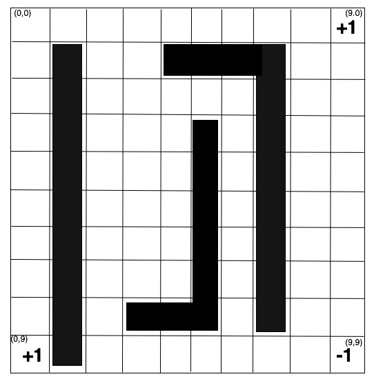
You may assume R=-0.04 for all non-goal states, and gamma = 0.8.
Here's an example of what the code looks like running in the Python interpreter:
>>> import mdp>>> m = mdp.makeRNProblem()
>>> m.valueIteration()
>>> [(s.coords, s.utility) for s in m.states.values()]
[(0, 0), (1, 0.30052947656142465), (2, 0.47206207850545195), (3,
0.68209220953458682), (4, 0.18120337982169335), (5,
0.34406397771608599), (6, 0.09080843870176547), (7,
0.095490116585228102), (8, 0.18785929363720655), (9,
0.00024908649990546677), (10, 1.0), (11, -1.0)]
>>> m.policyIteration()
>>> [(s.coords, s.utility, s.policy) for s in m.states.values()]
[(0, 0, None), (1, 0.28005761520403155, 'right'), (2,
0.4690814072745027, 'right'), (3, 0.68184632776188669, 'right'), (4,
0.15435343031111029, 'up'), (5, 0.34377291077136857, 'up'), (6,
0.061864822644220767, 'up'), (7, 0.088791721072110752, 'right'), (8,
0.18680600621029542, 'up'), (9, -0.00075615039456027738, 'left'), (10,
1.0, None), (11, -1.0, None)]
Select 1 of the following two problems to complete. You can get up to 40 points extra credit by completing both problems.
- Bayes
Networks & Message Passing
For this programming project, you will write a python program bayes.py that allows you to do inference in a Bayesian Network. For this assignment, you will only need to deal with trees (not polytrees), so each node will have a since parent (though nodes can have multiple children). Your program will read in the network (including link matrices and priors), a number of lambda messages (for observed variables), and will output the belief in each variable given all of the evidence.
The first line of the input file will be the number of variables in the system.
The next n lines of the input file (one for each variable in the system) will be of the form:
<variable name> <number of values for the variable>
After the description of the variables, there will be a link matrix for each variable, in the form:
P(<childname>|<parentname>)
<P(child = c1 | parent = p1)> <P(child = c2 | parent = p1)> ... <P(child = cj | parent = p1)>
<P(child = c1 | parent = p2)> <P(child = c2 | parent = p2)> ... <P(child = cj | parent = p2)>
...
<P(child = c1 | parent = pk)> <P(child = c2 | parent = pk)> ... <P(child = cj | parent = pk)>
(Assuming that the child has j values and the parent has k values)
Following the link matrices, there will be a line of 5 dashes:
-----
Followed by a list of evidence for a subset of the variables, of the form:
<variable name> <lambda(X=x1)> <lambda(X=x2)> ... <lambda(X=xk)
Followed by another line of 5 dashes:
-----
Your program will take as an iput parameter a filename, and print out the belief BEL(X) = P(X | evidence) for each variable in the network. If your program is called with the verbose flag (-v), then you will print out all the lambda and pi messages as well
A legal input file might look like the following:
3
B 4
Al 3
A2 3
P(A1|B)
1.0 0.0 0.0
0.5 0.4 0.1
0.06 0.5 0.44
0.1 0.4 0.5
P(B)
0.891 0.099 0.009 0.001
P(A2|B)
0.9 0.05 0.05
0.8 0.1 0.1
0.8 0.1 0.1
0.1 0.1 0.8
-----
A1 1 0 0
A2 0 0 1
-----
Which would produce the output:
% python bayes.py eg1
BEL(B) : [0.89757, 0.099730, 0.001088, 0.001612]
BEL(A1) : [1.000000, 0.000000, 0.000000]
BEL(A2) : [0.000000, 0.000000, 1.000000]
While the input file:
5
B 4
A1 3
A2 3
A3 2
M 2
P(M|A1)
0.9 0.1
0.2 0.8
0.1 0.9
P(B)
0.891 0.099 0.009 0.001
P(A1|B)
1.0 0.0 0.0
0.5 0.4 0.1
0.06 0.5 0.44
0.5 0.1 0.4
P(A2|B)
0.9 0.05 0.05
0.8 0.1 0.1
0.8 0.1 0.1
0.1 0.1 0.8
P(A3|B)
1 0
0.1 0.9
0.9 0.1
0.9 0.1
-----
A2 1 0 0
A3 0 1
-----
Would produce the output:
% bayes -v eg2
Variable B:
pi(B) :[0.891000, 0.099000, 0.009000, 0.001000]
lambda(B) :[0.000000, 0.720000, 0.080000, 0.010000]
BEL(B) :[0.000000, 0.989863, 0.009999, 0.000139]
Variable A1:
pi(A1) :[0.495601, 0.400958, 0.103441]
lambda(A1) :[1.000000, 1.000000, 1.000000]
BEL(A1) :[0.495601, 0.400958, 0.103441]
lambda_A1(B) :[1.000000, 1.000000, 1.000000, 1.000000]
pi_B(A1) :[0.000000, 0.989863, 0.009999, 0.000139]
Variable A2:
pi(A2) :[0.799223, 0.100000, 0.100777]
lambda(A2) :[1.000000, 0.000000, 0.000000]
BEL(A2) :[1.000000, 0.000000, 0.000000]
lambda_A2(B) :[0.900000, 0.800000, 0.800000, 0.100000]
pi_B(A2) :[0.000000, 0.988901, 0.009989, 0.001110]
Variable A3:
pi(A3) :[0.167514, 0.832486]
lambda(A3) :[0.000000, 1.000000]
BEL(A3) :[0.000000, 1.000000]
lambda_A3(B) :[0.000000, 0.900000, 0.100000, 0.100000]
pi_B(A3) :[0.000000, 0.915607, 0.083237, 0.001156]
Variable M:
pi(M) :[0.536576, 0.463424]
lambda(M) :[1.000000, 1.000000]
BEL(M) :[0.536576, 0.463424]
lambda_M(A1) :[1.000000, 1.000000, 1.000000]
pi_A1(M) :[0.495601, 0.400958, 0.103441]
Note that your output does not need to be exactly in this format, but it does need to contain the same information and be nicely formatted so that it is easy to read.
Calculating BEL(X)
You need to calculate BEL(X) for each variable X in the system. Since BEL(X) = αλ(X)π(X), you only need λ(X) and π(X) for each variable, which can be calculated in the following way (note that in the following descriptions, when multiplying a matrix and a vector use matrix multiplication, when multiplying or dividing two vectors use element-by-element multiplication or division):
Calculating λ(X):

Where λevidence(X) has the values in the input file (if there is evidence for that variable in the input file), or [1, 1, 1, ..., 1] otherwise.
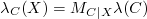
Calculating λC(X):
Calculating π(X):
If X is a root variable, then π(X) = Prior Probability of X, as read from the input file
If X is not a root variable, then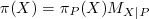 ,
where P is the parent of X.
,
where P is the parent of X.
Calculating πP(X):

Alternately,
πP(X) = BEL(P) / λX(P)
Some Hints:
Calculate the λ messages first, then calculate the π messages.
Calculate the λ messages bottom-up. That is, first calculate the λ messages for the leaves, then the parents of the leaves, and so on. A topological sort may help you here.
Calculate the π messages top-down. That is, first calculate the π messages for the root, then the children of the root, and so on. Again, a topological sort may help you here.
Program Decomposition is your friend: Test each piece in isolation before trying to put everything together. Make sure you read in the data file correctly, and compute the parents of each node correctly. Get the matrix multiplication working,
and then the topological sort, then do λ messages, then do π messages.
You might try simpler problems before moving on to more complex problems. Try chains before moving on to trees.
Some files to get you started are here: bayes.py
Another test file:
bayesTest, bayesOutput
- Bayes
Networks: Monte Carlo
For this project, you will write a program that does inference in a (non-polytree) Bayesian network using the Monte Carlo method. For simplicity, you can assume that all of the variables are binary. The input file is similar to (but not exactly the same as) the input file for message propagation
The first line of the input file will be the number of variables in the system.
The next n lines of the input file (one for each variable in the system) will contain the variables in the system
After the description of the variables, there will be a link matrix for each variable. For variables that have no parents, the link matrix will be of the form:
P(<variable name>)
<P(<variable name> = false)> <P(<variable name> = true)>
For instance, if A is a root variable that is true with probability 0.66, we would have:
P(A)
0.34 0.66
For a variable with two parents A and B, the link matrix:
P(A|B,C) not a a not b, not c 0.2 0.8 not b, c 0.5 0.5 b, not c 0.3 0.7 b, c 0.4 0.6
Would be represented as:
P(A|B,C)
0.2 0.8
0.5 0.5
0.3 0.7
0.4 0.6
Likewise, for a variable A with three parents B, C, and D, the link matrix:
P(A|B,C,D) not a a not b, not c, not d 0.2 0.8 not b, not c, d 0.5 0.5 not b, c, not d 0.3 0.7 not b, c, d 0.4 0.6 b, not c, not d 0.1 0.9 b, not c, d 0.8 0.2 b, c, not d 0.6 0.4 b, c, d 0.9 0.1
Would be represented as:
P(A|B,C)
0.2 0.8
0.5 0.5
0.3 0.7
0.4 0.6
0.1 0.9
0.8 0.2
0.6 0.4
0.9 0.1
Following the link matrices, there will be a line of 5 dashes:
-----
Followed by a list of evidence for a subset of the variables, of the form:
<variable name> <value>
Followed by another line of 5 dashes
A legal input might look something like the following:
4
A
B
C
D
P(A)
0.3 0.7
P(B|A)
0.8 0.2
0.3 0.7
P(C|A)
0.9 0.1
0.2 0.8
P(D|B,C)
0.1 0.9
0.6 0.4
0.7 0.3
0.9 0.1
-----
D 1
-----
Your program will take as input the number of iterations, and a filename, and will run the appropriate number of trials. For each trial, you will pick a value for each of the variables, based on the link matricies. For root variables, select a value based on the probability that the variable is true. given the priors stored in the link matrix. For variables with parents, look at the values selected for all parents, and then use the appropriate row in the link matrix to determine the value for the variable. When you are done, see if the evidence matches your values. If it does not, throw out the trial. If it does, then record the frequencies that each variable is true. When all the trials are done, the belief in each variable is the number of times that variable was true / valid trials.
Note that we are only doing very simple queries -- things like P(a | b, c) -- not anything complicated like P(a,b | c,d).
Your program should output:
# of valid trials
probability for each variable
For the above input file, and 100000 trials, you might get something like:
Valid Trials: 39759
P(A) = 0.436
P(C) = 0.292
P(B) = 0.216
P(D) = 1.0
Note that your numbers may be somewhat different.
Some files to get you started:
montecarlo.py